Master Ggplot2: Your Cheat Sheet For R Data Visualization
Are you striving to unlock the secrets of compelling data visualization? Mastering `ggplot2`, R's powerhouse package, is your key to transforming raw data into insightful and engaging visual narratives.
In the dynamic realm of data analysis, the ability to communicate findings effectively is paramount. Data visualization is no longer a supplementary skill; it's a core competency. And when it comes to creating polished, informative, and aesthetically pleasing graphs, `ggplot2` reigns supreme. This article delves into the core concepts, providing a roadmap for both novice and seasoned users to harness the full potential of this remarkable package. Whether you're a student, a researcher, a data scientist, or simply someone curious about the power of data visualization, this guide will equip you with the knowledge to craft compelling stories from your data.
At its heart, `ggplot2` is built upon the 'grammar of graphics.' This foundational concept posits that any graph can be constructed from a series of standardized components: a dataset, a coordinate system, and 'geoms' - the visual elements that represent data points. But, more than just a set of building blocks, `ggplot2` offers a philosophy. It emphasizes a layered approach, enabling you to build plots iteratively, adjusting and refining each component until you achieve the desired visual outcome.
- Tyla Unveiling The Rising Star Her Music Journey
- Mr Tumble Allegations Controversy What You Need To Know
Let's decode the core of `ggplot2`. Heres a simple summary of the basics:
- Data: The foundation of any visualization. This is the data you want to represent, typically structured as a data frame.
- Geometries (Geoms): These are the visual representations of your data. Examples include points (`geom_point`), lines (`geom_line`), bars (`geom_bar`), and boxplots (`geom_boxplot`).
- Aesthetics (Aesthetics): These are the visual properties that map data variables to visual attributes. This includes things like the position (`x`, `y`), color (`color`), fill (`fill`), shape (`shape`), size (`size`), and transparency (`alpha`) of your geoms.
- Scales: Control the mapping of data values to the visual properties. For example, you may want to use a linear scale for a continuous variable, or a discrete scale for categorical data.
- Coordinates: Determine how the data is displayed. Common options include the Cartesian coordinate system (the standard x-y axes), polar coordinates, and more.
- Facets: This allows you to create multiple small plots based on the levels of a categorical variable.
- Themes: Control the overall look and feel of your plot, encompassing elements like background color, grid lines, and text formatting.
Below is a table summarizing some of the main geoms and their parameters which is useful for creating a wide variety of charts, adjusting colors, labels, axes, legends, annotations, and more.
| Geom | Description | Key Parameters | Example |
|---|---|---|---|
geom_point() | Creates a scatterplot, representing data points with individual dots. | x, y, color, shape, size, alpha | ggplot(data, aes(x = var1, y = var2, color = group)) + geom_point() |
geom_line() | Draws a line connecting data points, often used for trends over time. | x, y, color, linetype, size | ggplot(data, aes(x = time, y = value, group = id)) + geom_line() |
geom_bar() | Creates bar charts, representing frequencies or counts of categorical data. | x, y, fill, color, width | ggplot(data, aes(x = category, y = count, fill = category)) + geom_bar(stat ="identity") |
geom_histogram() | Displays the distribution of a single continuous variable using bins. | x, fill, color, binwidth, bins | ggplot(data, aes(x = value)) + geom_histogram(binwidth = 10) |
geom_boxplot() | Visualizes the distribution of data through quartiles, median, and outliers. | x, y, fill, color, width | ggplot(data, aes(x = group, y = value, fill = group)) + geom_boxplot() |
geom_density() | Displays the smoothed distribution of a continuous variable. | x, fill, color, alpha | ggplot(data, aes(x = value, fill = group)) + geom_density(alpha = 0.5) |
For more detailed information, consider consulting ggplot2 documentation.
- Pineapplebrat Leaks Latest Nudes Videos Onlyfans Instagram
- Zach Woods Relationship Status Single Or Married
The real power of `ggplot2` emerges from its ability to customize plots. The core functions and arguments, along with the flexible use of aesthetics, allow data scientists to create visually compelling graphs that effectively communicate complex information. Moreover, `ggplot2` supports data manipulation seamlessly, allowing you to transform your data within the plotting code itself, reducing the need for extensive pre-processing. This flexibility is vital to produce the visualization best suited to the nature of the dataset.
Let's talk about building a plot. Every graph begins with a call to the `ggplot()` function, where you provide the data and specify the aesthetic mappings using `aes()`. These mappings define how the data variables will be translated into visual properties like position, color, shape, and size. Think of `aes()` as the map between your data and the visual elements of the graph.
After initializing `ggplot()`, you then add layers using the `+` operator. Each layer represents a geometric object (`geom`), such as points, lines, or bars. Within each `geom`, you can further customize the aesthetics, overriding or adding to the initial aesthetic mappings defined in the `ggplot()` call. This layering system allows you to build complex plots incrementally, adding or modifying elements as needed.
Scales play a crucial role in the appearance and interpretation of your plot. They control how the data values are mapped to the visual properties. `ggplot2` provides a wide range of scales for different data types and visual attributes. For continuous variables, scales like `scale_x_continuous()` and `scale_y_continuous()` are used, offering options to adjust the axis limits, breaks, labels, and transformation. Categorical data utilizes scales such as `scale_color_discrete()` and `scale_fill_brewer()`, enabling you to customize colors and ensure consistent visual representation across categories.
Coordinate systems determine how the data is positioned within the plot. The most common is the Cartesian coordinate system, where data points are displayed based on their x and y values. Other coordinate systems, like polar coordinates, are useful for creating specialized visualizations such as pie charts or radar charts. To adjust the coordinate system, use the `coord_ ()` functions. For instance, `coord_flip()` can be used to flip the x and y axes, creating a horizontal bar chart, and `coord_polar()` allows you to create polar charts.
Facets enable the creation of small multiples, allowing you to display multiple plots side-by-side based on the levels of a categorical variable. This technique is invaluable for comparing the distributions of a variable across different groups or time periods. The `facet_wrap()` and `facet_grid()` functions are the key to faceting in `ggplot2`. `facet_wrap()` wraps the plots into a 1D or 2D arrangement, while `facet_grid()` creates a grid where you can specify the rows and columns based on the levels of your categorical variables.
Themes in `ggplot2` control the overall aesthetic style of the plot. They encompass elements like background color, grid lines, font sizes, and legend appearance. By changing the theme, you can instantly transform the look and feel of your plot. `ggplot2` provides a variety of built-in themes, such as `theme_bw()`, `theme_classic()`, and `theme_minimal()`. You can also customize themes extensively using the `theme()` function, providing granular control over individual elements of the plot.
Annotations are a critical component of effective data visualization, allowing you to highlight specific data points, add labels, and provide context to the plot. `ggplot2` provides various functions to add annotations to your plots. For simple text annotations, you can use `geom_text()` or `geom_label()`. For more complex annotations, such as arrows, lines, or rectangles, you can use functions like `geom_segment()`, `geom_vline()`, and `geom_rect()`. Adding annotations can guide the viewer's attention and emphasize key insights.
Legends are automatically generated in `ggplot2` based on the aesthetic mappings you define. However, you can customize the legend's appearance and behavior using the `guides()` function. You can control the title, labels, position, and appearance of the legend. For example, you can change the legend title using `guides(color = guide_legend(title ="My Title"))`. You can also suppress the legend for certain aesthetics, such as `guides(fill ="none")`, if you don't want to include it in the plot.
Beyond the fundamental components, `ggplot2` offers a range of specialized techniques for creating even more sophisticated visualizations. Consider these advanced capabilities:
- Statistical Transformations: `ggplot2` offers built-in statistical transformations (stats) that can calculate values like counts, proportions, and smoothed densities directly within the plot. The `stat_()` functions allow you to perform these transformations without the need to pre-calculate them.
- Interactive Plots: While `ggplot2` itself creates static plots, you can integrate it with interactive visualization libraries, such as `plotly`, to create dynamic and engaging visualizations. These libraries add features like tooltips, zooming, and panning, enhancing the exploration of the data.
- Custom Geoms: If the built-in geoms do not meet your needs, you can create your own custom geoms. This requires a deeper understanding of the grammar of graphics but gives you the flexibility to visualize data in innovative ways.
To summarize, `ggplot2` is a comprehensive and powerful tool for data visualization, built on a robust foundation of the grammar of graphics. Its layered approach, extensive customization options, and integration with the R ecosystem make it an invaluable asset for anyone working with data. By mastering the basics data, geoms, aesthetics, scales, coordinates, facets, and themes and exploring the advanced techniques, you can unlock the full potential of `ggplot2` and create impactful and informative visualizations that tell compelling stories with data.
- Explore Wasmo Somali Channels Find Your Favorites
- Park Boyoungs Relationship Timeline Dating History Rumors Explained
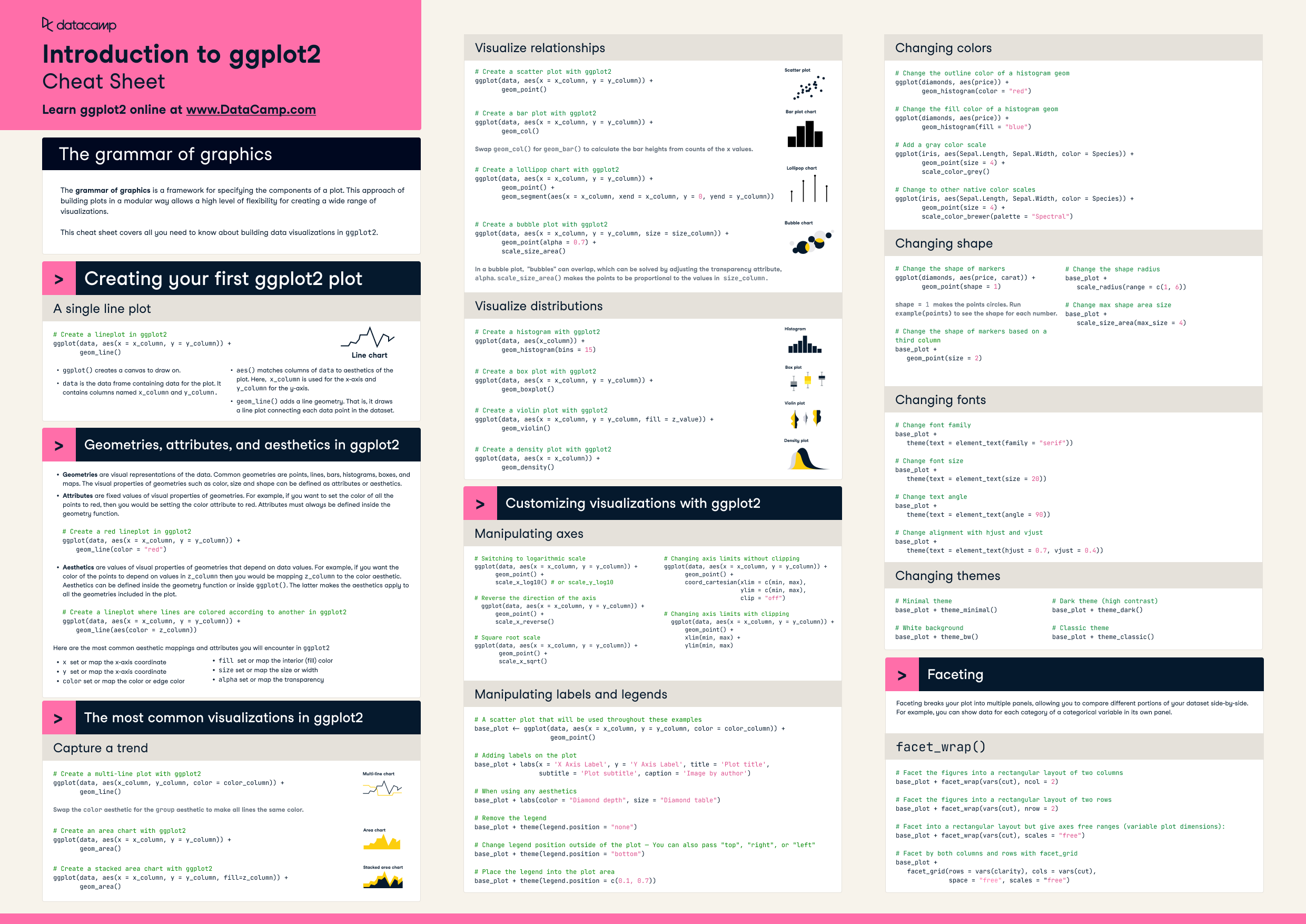
ggplot2 Cheat Sheet DataCamp

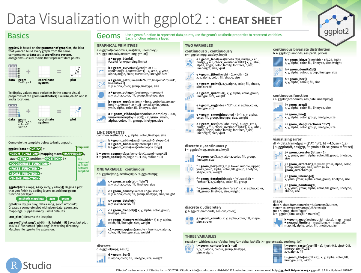
Ggplot2 Cheat Sheet Data Visualization Machine Learning Data Vrogue
How to make a plot with two different y axis in R with ggplot2? (a
